
I’ve spent the last few weeks writing my first ever fellowship proposal, which has been an interesting new kind of writing for me! One of the aspects of writing persuasively about my science was planning out the figures - I found myself thinking about the points that my diagrams made in the overall argument a lot more than I would have otherwise.
Of interest to us today is one figure where I talked about the dynamical processes taking place in clouds, by way of illustrating why it was a really complicated problem with a lot of things interacting. I’m leaving out the actual figure because I’ll probably want to use it in a paper or something later, but the only relevant factors are: I was making it in PGF/TikZ, LaTeX’s language for graphics based on coordinate specifications; and I wanted to put a border around the whole thing in the shape of a cloud.
TikZ actually has a builtin cloud shape, so this seemed simple at first:
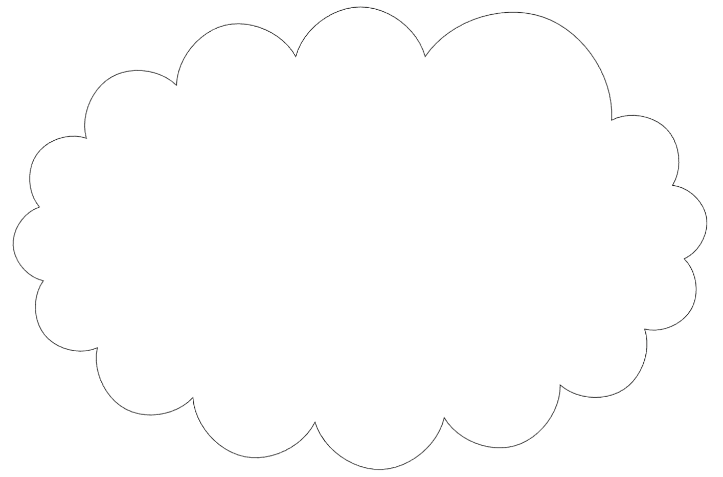
But this has a few problems. Between each loop, you have a sharp corner, which didn’t feel very good. Also, it’s up-down symmetric, but actual cloud profiles are a bit thicker at the bottom and drop off to the top, because cloud particles fall down due to gravity and more of them are kept aloft at lower positions. More practically from a figure design perspective, I didn’t like the idea of needing to compress text to accommodate the sharp corners, or allowing extra space for a puffy border both on the bottom and the top.
So I set about trying to draw my own cloud! I’m not very artistically inclined; I have a vivid memory of failing an art exam as an 8-year-old, because I had to draw a shoe and I ran through about 40 pieces of paper staring at my own shoes and trying to get the perspective right. Maybe I was overthinking it, but if that’s the case I don’t see any reason I should stop now.
One of the reasons I like TikZ is it’s very declarative; if you look at something and think “that seems wrong”, there’s a fixed set of things you can vary until it looks right. (I say I like it, but before this proposal I hadn’t actually done all that much with it, and that’s because my preferred way of making diagrams is not to make them. But it’s all part of my evolution as a scientist!) In this case, I felt I could reduce this down to a math problem: there’s some sort of parametric curve creating this shape with the sharp corners, and I have to make another one that didn’t have it. Simple, right?

TikZ has a built-in structure for making smooth curves based on control points, and from animations I’ve found online it seems like it does this using cubic Bézier curves. You pick a start and an end point, pick two control points setting (roughly, I think) initial and final velocities of the curve, and TikZ will draw a smooth curve connecting those end points that get “pulled” towards the control points.
\draw[] (0.0, 3.0) .. controls (1.0, 3.5) and (2.0, 2.5) .. (3.0, 3.0);
To me this seemed like the perfect recipe for a cloud: I’d vary the control points till I got a shape for a single loop that was satisfactorily cloud-like to my eye, and then I’d repeat that throughout the whole cloud.
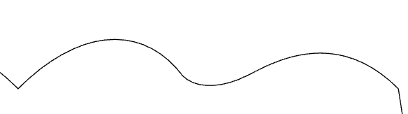
The issue I ended up running into there - in addition to having to track a bunch of additions/subtractions of coordinate numbers in my head - was velocity continuity. I could make a curve that looked convincingly enough like a little loop of a cloud, but I had to join the end of that curve up with the start of the next one to make the next loop. If I didn’t make a straight line with my control points across the curves, I’d get a weird-looking join. (This is explained in a lot more mathematical detail in two excellent videos by Freya Holmér.) Here, I was able to smooth it out at the interface of two loops for one little bit, but to the left and off to the side where I was forming the right edge, any control point manipulation would mess up the join I’d just fixed. In hindsight, plotting the control points and visualizing it as if I was moving the velocity vectors would’ve been helpful, but I like the approach I ended up with better.
So it seemed like I was stuck - if my first control point was fixed, I couldn’t use it to make the thing that I intuitively understood to be a cloud shape. The problem of deciding where the control points should be was starting to sound very analytical.
If anyone who advises me happens to be reading this, please don't pay any attention to the timestamps and how close they were to the deadline.
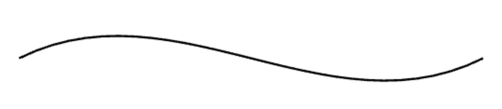
I decided to step back a bit - let’s figure out what the overall curve should look like, then we can try and decide on control points that reproduce that curve. We want an individual loop to have a big peak out, and a small peak in, and vary smoothly the whole time. I figured I shouldn’t try to solve for this expression over the cloud path just yet - instead, we’ll assume we want this variation over an interval $t \in [0, 1]$, which we can interpret as the “time” parameter in a parametric curve. Later, we’ll start with a baseline shape and add cloud loops over the top of it by appropriately rescaling, reshaping, and repeating this little function, but at its most basic level, we just want a function $f: [0, 1] \to \mathbb{R}$.
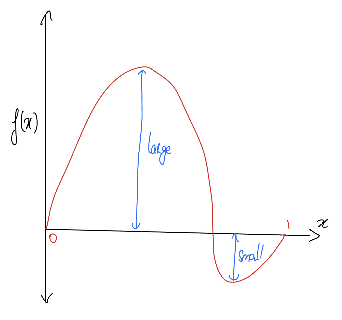
I probably want this to be two sine waves stuck together, because it seems like what I’ve just described is a sine wave where it changes amplitude halfway through. The trick is going to be making sure that it’s continuous and avoids the weird-looking joins we saw before. I started writing down the constraints and realized I’d basically made up a Calc 1 problem!
Let’s figure out what this should do. I want something that’s one sine wave up to some point, and another one after that point:
\[f(x) = \cases{\sin(\omega_1 x) & x < a \\ \sin(\omega_2 x) & x >= a}\](For some reason MathJax doesn’t like $\geq$ in the cases framework, oh well.)
We want to choose $a < 1$ so that we actually reach this crossover point. We’ll set $a$ to at least $1/2$ because we want the first peak to be the larger one and for it to take up most of the space, but we’ll leave room to tune it later. Since we want the second peak to be negative, and smaller than the first one, we’ll introduce a new variable $r$ satisfying $0 < r < 1$ that gives us the relative amplitude. We can fix the amplitude of the first peak equal to 1, and we’ll rescale the whole shape later if we have to.
\[f(x) = \cases{\sin(\omega_1 x) & x < a \\ - r \sin(\omega_2 x) & x >= a}\]We’re fine with the first one starting at 0 when $x = 0$, but for the second one, we want it to hit 0 and to be moving down when $x = a$. Since we’re not sure how to do this yet, we’ll add a phase offset $\varphi$ and figure out what it should be later.
\[f(x) = \cases{\sin(\omega_1 x) & x < a \\ - r \sin(\omega_2 x + \varphi) & x >= a}\]There’s five free parameters here: $\omega_1$, $\omega_2$, $a$, $r$, $\varphi$. Some of these are going to be set by our continuity conditions, but we can immediately see that some will remain free for us to customize how we want our cloud to look. As an example, look at the case where $a = 1/2$; you’re halfway through the wave at the halfway point, so all the other parameters should line up to make the same full sine wave. Since we were free to set $a$ without it inducing an inconsistency, we have a sense we’ll probably be able to vary at least one parameter later on.
Let’s put down some constraints! First, what points should it pass through?
- At $x = 0$, we should have $f(0) = 0$. This is already fixed because I didn’t allow for a phase on the first component.
- At $x = a$, we should have $\lim_{x \to a^-} f(x) = 0$. In general there’s some degeneracy in how you get to this because the solution for $sin(x) = 0$ is $x = n\pi, n \in \mathbb{Z}$, but I only want one half-wave till we get to $x = a$. So the argument should be $\pi$, giving us the constraint $\omega_1 a = \pi$. Since $\omega_1$ only shows up here, I’ll eliminate that.
- At $x = a$, we should also have $\lim_{x \to a^+} f(x) = 0$. This is more subtle because it’s evaluated at $a$ and not 0. I’m going to dodge this by getting rid of the $\varphi$ and instead changing the argument to $\omega_2 (x - a)$ so that we have the same kind of “automatic elimination” of the phase as in the first point.
Let’s look at what this leaves us with:
\[f(x) = \cases{\sin(\pi x / a) & x < a \\ -r \sin(\omega_2 (x - a)) & x >= a}\]We’ve got it down to three variables, but there’s still more to constrain. We have one more point-based constraint:
- At $x = 1$, we should have $f(1) = 0$, and once again we want that to be at a phase of $\pi$. This means we want $\omega_2(1 - a) = \pi$, so substituting this back in, we get
Alright, maybe we’re done? We have two parameters left: $a$, the location of the zero crossing, and $r$, the amplitude of the second (negative) peak. Maybe we have freedom in both of those.
Not quite. We haven’t addressed the problem of the joins being in the right place but being awkward. Here’s a GIF I made in Desmos where I fix $a = 0.8$ and sweep over $r$.
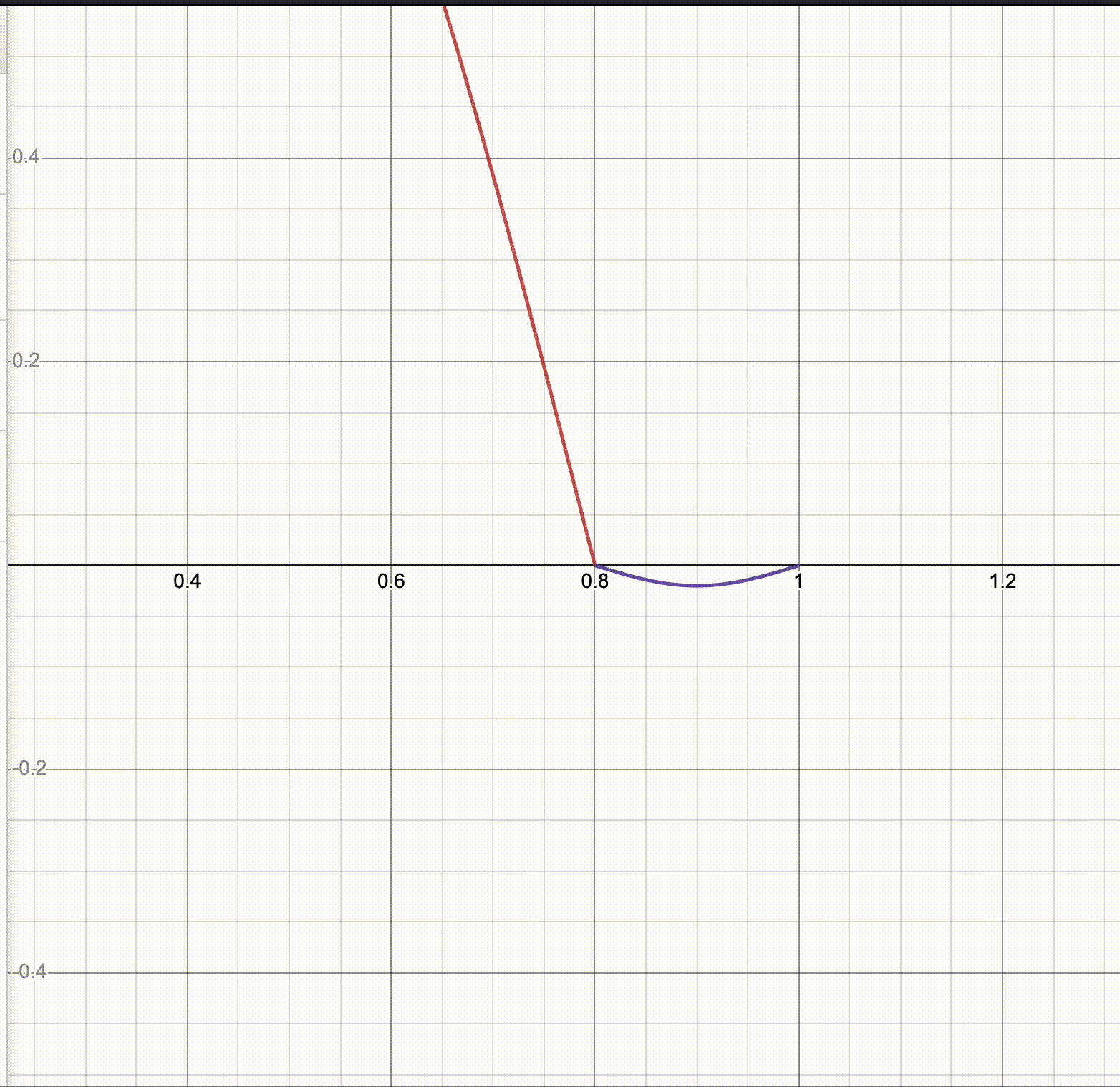
It seems like there’s a critical point at which you have a smooth-looking join, and if you just freely vary $r$ it’ll either be too shallow or too steep for that. So there’s one more constraint.
You can also anticipate this algebraically; all of the constraints I’ve applied so far are saying the function value at some point should be 0. That means we’re independent of the overall scale; you can multiply both components by different things and all the constraints we’ve put down will still hold, but by eye we absolutely see when the scales are incongruous.
We can put this idea of smoothness into our algebra by saying we have to make sure the two functions share a tangent line at the join. That is, their derivative is continuous, or the same at the left and right of the join:
\[\lim_{x \to a^-} f'(x) = \lim_{x \to a^+} f'(x).\] \[\left.\frac{\mathrm{d}}{\mathrm{d}x} \sin(\pi x / a) \right|_{x = a} = -r \left.\frac{\mathrm{d}}{\mathrm{d}x} \sin\left(\pi \frac{x - a}{1 - a}\right) \right|_{x = a}\] \[\frac{\pi}{a} \cos(\pi) = -r \frac{\pi}{1 - a} \cos(0)\]$\cos(\pi) = -1$ and $\cos(0) = 1$, so the negatives, cosine values, and $\pi$s all cancel:
\[\frac{1}{a} = r \frac{1}{1 - a} \implies r = \frac{1}{a} - 1 \implies a = \frac{1}{1 + r}.\]Let’s check if this is a reasonable answer by substituting in some edge cases:
- If $a = 1/2$, $r = 1$. This is the case we looked at earlier: if you reach a half-turn of phase halfway through, you should just follow through on the same sine curve, with the positive and negative peaks having the same amplitude. This is what we see!
- If $a = 1$, $r = 0$. You only have time for a half-turn and the second peak doesn’t get any amplitude.
Seems good! I’ll leave the equation above as it is though, because substituting it in gets messy. You can play around with this in Desmos here.
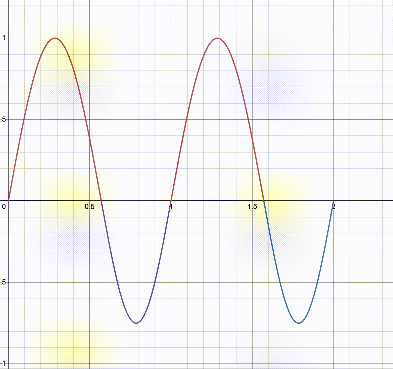
Here’s a bunch of the resulting curves on one plot (with I think $1/r$ on the legend, for convoluted reasons that only the late-night programming brain can come up with):
And the derivative curves! Julia’s autodiff is so nice, I barely had to change anything compared to the last plot to generate this. You’ll notice that the derivative shows a non-smooth join, which is because we didn’t have any free parameters with which to match up the higher-order derivatives. If we’d tried to enforce second-derivative continuity, we’d be forced to set $a = 1/2$ and we’d be stuck with pure sine waves.
You may ask: “how did we get continuity at $x = 1$? We only enforced it at $x = a$, but there’s a join at each integer as well, and we didn’t do anything to make sure those ones were smooth.” This actually gets enforced automatically when you set it for $x = a$! You can find this out algebraically, but a quicker argument runs: $x = a$ links the end of the first curve (at a $\pi$ phase shift) to the start of the second (at a 0 phase shift), and at $x = 1$ the roles get switched, with the first curve at a 0 phase shift and the second at a $\pi$ phase shift. So both derivatives get phase-shifted by $\pi$, which for sin and cos is a sign flip, meaning they’ll still match up and you have the same slope, just in the opposite direction.
Okay, for a more pertinent example, you may ask: “what does any of this have to do with clouds?”
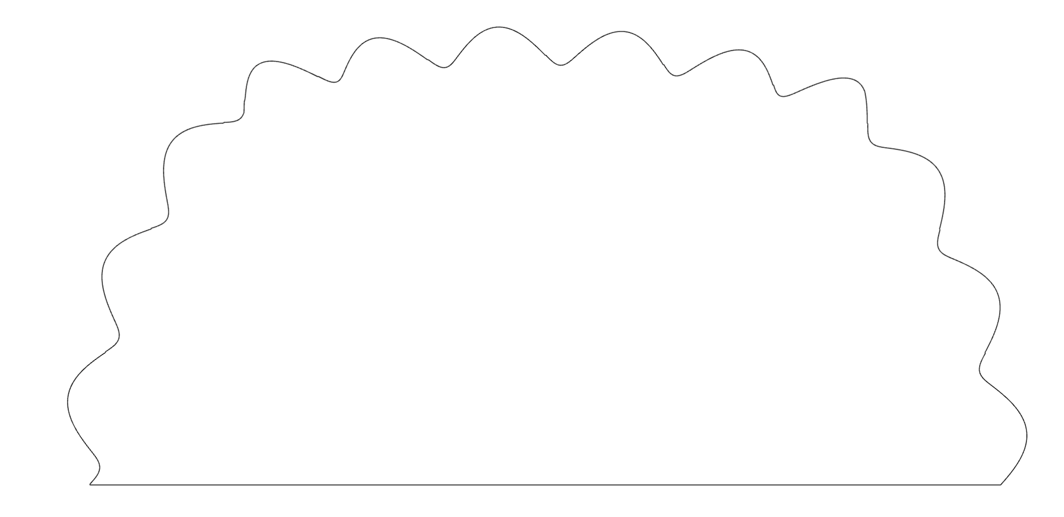
I’ll put this curve back onto some sort of base figure and loop it around several times. I started with a half-ellipse, which I got by evaluating $x = a \cos(\theta), y = b \sin(\theta)$ for some arbitrarily-chosen $a, b$ that looked nice and for $\theta$ sampled finely between 0 and $\pi$. I added my loops as a perturbation: splitting up the $\theta$ range into $n$ intervals of size $\pi / n$ each, I took my two-sine-wave curve (with $r = 1/7$) and scaled it by $\cos(\theta)$ for the $x$ component and $\sin(\theta)$ for the $y$, and added it to the curve. Here’s the result! The orange trapezium (or trapezoid if I’m to accept I’ve become fully American now) was a guiding footprint for the content I wanted to put inside the cloud.
We have a curve! Now I had to put it back into TikZ, which meant identifying control points. My first idea was to pick every point where the curve changes direction:
Unfortunately, this didn’t work too well. I’m sure I could think through why that happened more carefully and pick better control points - off the top of my head, since they set the velocity vectors, I think they don’t necessarily have to be on the path. But I realized PGF had a function to trace out a smooth curve connecting arbitrary numbers of points, so I just sampled the curve really finely, saved it to a text file, and read that into my LaTeX document.
All the remaining adjustments were to make sure it fit the text properly and didn’t take up too much space. It turned out my ellipse should be nearly a circle to fit everything in, but that left a lot of room at the top of the cloud, so I had to change the base figure:
And after a lot of tweaking things and rearranging where my content went within the cloud, I settled on this (with fun science content inside):
I put it into my proposal document, stepped back, and went “…I don’t really like this.” In the context of the proposal, it just didn’t seem to fit, and it pushed me over my page limit. So after many hours of working out math and coding across Julia and TikZ, I just threw it out. I might bring it back on another occasion, but it felt wrong in this case.
I could justify this whole experience by saying it’s helpful to look at alternative forms of my figures so I can find out what does and doesn’t work, and I believe that to some extent. But honestly, it was just a fun puzzle. I’ve found that since I started doing research full-time, any fun puzzles I come across get folded into the larger research project, so I have to save this kind of writeup for a formal research product like a paper or presentation. I liked getting to just solve something in one sitting and work through just enough hurdles to keep it interesting but not frustrating!