
I like solving Sudokus, but I’m not that great at them - my strategy mostly involves the following steps:
- Fill in anything I see immediately.
- Stare at the puzzle for ten to thirty minutes before I see something else.
- Repeat 1-2 till solved.
This isn’t a very satisfying way to do a puzzle, so I set out to understand it better by writing a program that implements my method! In this way, I can hopefully figure out what it is I’m seeing, and develop some new ways of solving puzzles.
While there’s fast Sudoku solvers out there already, I’ve got a more specific goal with mine: to generate a list of steps that a human could follow to see the path to the solution. It’s possibly most natural to a computer to express Sudoku as a boolean satisfiability or integer programming problem, but that’s not how a human would think about it. There’s also articles out there on how to solve them algorithmically, but I won’t consult them either except for images. The journey’s more important to us than the destination!
I’ll be using the Julia programming language and pasting code snippets here, but hopefully nothing depends too heavily on language specifics. If you’d like to run the code, take a look at the GitHub! My code snippets here will be out of order and messy for the purposes of actually running anything, so it’s best to look on there, where I’ve structured it better and it’ll be actually runnable.
Setting everything up
As a quick refresher, a Sudoku consists of a 9x9 grid, subdivided into nine 3x3 blocks, with cells each containing one of the integers 1-9. In the completed puzzle, each column, row, and block contains each of the integers 1-9 exactly once. Solving the puzzle consists of repeatedly applying constraints (“I’ve got 1, 2, 4, 5, 6, 7, 8, 9 in this row, and one space left, so it has to be 3” and so on) until all 81 cells have been filled.
We’re trying to express this in code, so let’s start off with a matrix representing the board.
We’ll use the convention that if a cell is empty, that’s represented in the matrix by a 0.
If we print this, we’ll get a 9x9 grid of numbers separated by spaces - not bad, but I’d like to separate out the blocks and see the puzzle more cleanly. So let’s add in a function to make printing a bit more legible!
To do this, I can go row by row, column by column, and print each number, except:
- At the end of each row, I want to move to a new line
- Every third number in a row, I want a vertical separator
| - After every three rows, I want a row of horizontal separators -
For that, I want to go over each row (counting as I go), and within that each element (also counting as I go), printing, and doing something extra. After a little experimenting with the spacing, I got all of it:
This lets me look at the puzzle in my terminal like this!
julia> p = Sudoku([
           9 3 0 0 0 0 0 4 0
           0 0 0 0 4 2 0 9 0
           8 0 0 1 9 6 7 0 0
           0 0 0 4 7 0 0 0 0
           0 2 0 0 0 0 0 6 0
           0 0 0 0 2 3 0 0 0
           0 0 8 5 3 1 0 0 2
           0 9 0 2 8 0 0 0 0
           0 7 0 0 0 0 0 5 3
           ]);

julia> p
  -----   -----   -----
| 9 3 - | - 5 - | - 4 - |
| - - - | - 4 2 | - 9 - |
| 8 - - | 1 9 6 | 7 - 5 |
  -----   -----   -----
| - - - | 4 7 - | - - - |
| - 2 - | - - - | - 6 - |
| - - - | - 2 3 | - - - |
  -----   -----   -----
| - - 8 | 5 3 1 | - 7 2 |
| - 9 - | 2 8 - | - - - |
| - 7 - | - 6 - | - 5 3 |
  -----   -----   -----
Identifying solved puzzles
We could jump into solving from here, but first, let’s figure out when to stop. How does our program know when a puzzle is done? A quick way is to just check that there’s no 0s anywhere, but if that’s all we did, we could get false positives: maybe we filled in something wrong, but the program would mark it as correct because we put in a non-0 value there. Instead, we want to check that each (row, column, block) has all of 1-9 in it as well as there being no 0s.
An easy way to do this kind of check for duplicate values is to pass the subarray into a set, which removes any duplicates, and check that the size of that set is the same as that of the subarray. This gives us our first “check” method that we can call on any sub-region, and we can get the main one just by iterating over that first method for all rows, columns, and blocks.
To iterate over blocks, I added a new method named eachblock analogous to eachrow and eachcol that does what it sounds like. I’ll skip over how it works, but take a look on the main GitHub if you’d like!
By having two methods with the same name but different arguments, I’m using a Julia feature called multiple dispatch - here this mostly helps me with legibility/natural naming, but in other cases it can make the functionality better too!
Solving techniques
Now for the main event! We start off with a grid with some 0s and some known numbers in it, and we have to figure out how to substitute in the real numbers. That means applying constraints the way we manually do it.
There’s two ways I figure out a number in a Sudoku:
- For a particular cell, is there only one possible value?
- In a particular region, is there only one cell that could have a certain value?
  -----   -----   -----
| 9 3 - | - 5 - | - 4 - |
| - - - | - 4 2 | - 9 - |
| 8 - - | 1 9 6 | 7 - 5 |
  -----   -----   -----
| - - - | 4 7 - | - - - |
| - 2 - | - - - | - 6 - |
| - - - | - 2 3 | - - - |
  -----   -----   -----
| - - 8 | 5 3 1 | - 7 2 |
| - 9 - | 2 8 - | - - - |
| - 7 - | - 6 - | - 5 3 |
  -----   -----   -----
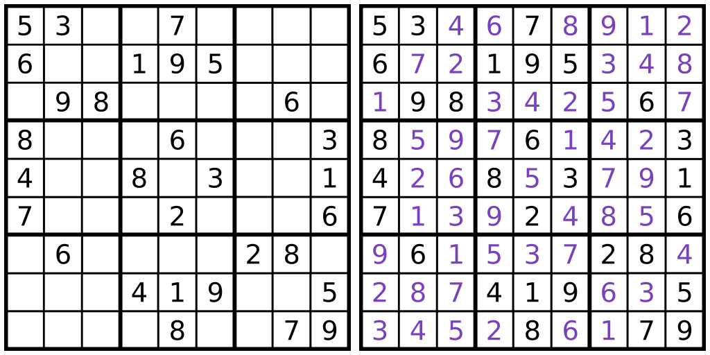
To illustrate both of these, let’s take a look at the puzzle I brought up earlier.
For the first constraint, the cell in the top-middle of the top-middle block (above the 4 which is itself above the 9) can only be a 5. We can eliminate 1, 2, 4, 6, 9 because they share a block, which leaves 3, 5, 7, 8. Looking down the column, we see a 3, 7, 8 (and an extra 3 in the row for good measure), meaning there’s no possibilities for that square other than 5. This second constraint is how we’ll start solving the puzzle really fast as soon as we’ve made some progress: as we fill in more, the possibilities for each cell get whittled down, and soon every cell can be filled in for sure!
An example of the second constraint would be: the only cell in the middle block that could be a 6 is the lower left one. There has to be a 6 somewhere in there, but it can’t be in the middle row because of the 6 in the center of the middle-right block, and it can’t be in the rightmost column because of the 6 in the bottom-right of the top-middle block. So there’s only one cell remaining. (If you’d like, try and spot some more constraints like this!)
So how do we tell our program to do this? It’s helpful to think of the overall logic before we get into details. When we’re writing a function called “solve”, we might want it to do something like this:
- Start with a grid
- Apply constraint 1 to fill in all forced values in a region
- Apply constraint 2 to fill in all forced cell values
- Return what we get
This is a good start, but we really want to apply both constraints multiple times: each time we apply the constraints, we get more information, and that can help us narrow down more possibilities.
- Start with a grid
- Loop:
- Apply constraint 1 to fill in all forced cell values
- Apply constraint 2 to fill in all forced values in a region
- Return what we get
When do we end this loop? We could say when the puzzle’s solved, i.e. when our “check” function returns true, but maybe we run into some puzzles where this won’t do it, and in those cases we would infinitely loop. There’s a few different ways to avoid this. What I went with is adding in a boolean that keeps track of whether we actually added any new values in a loop, and returning what we have if we didn’t. This covers both our cases: If we’ve got a complete puzzle, we won’t add anything in our last loop, because there’s nothing to add. If we’re stuck and can’t figure out anything more, this’ll successfully catch that and return us out.
This gives us the code for our first solver:
Writing the constraints
Now we have to implement the two constraints! To start with the first one, I wrote a function that gets the list of possible values given a cell index using the rule:
- If it’s already filled in, the only possibility is the actual value
- If it’s 0, then the possible values are 1 to 9
- minus any values in the row
- minus any values in the column
- minus any values in the block.
From there, writing the first constraint just needs us to loop over every cell (indices 1 to 9 along the rows and the columns).
The second constraint is trickier, and it took me a few iterations of trying out index combinations and different designs before I got one that worked. To start with, we know we’re doing this check for each region (row, column, block), so we should loop over those.
Within that, we’ll make use of our “possibilities” function again. For each of the nine cells in our region, let’s list the possibilities, and see if there’s any value that only shows up in one spot. To do that, I’ll make a possibilities matrix, where each cell in the matrix is itself a vector of the possible values. That sounds confusing, so here’s a possible top-left corner of this matrix:
    [1]     [2, 3, 9]    [3, 5, 8]
    [6]     [2, 7, 9]    [5, 7, 8]
    [3, 8]  [2, 3, 4, 9] [3, 8]
In this puzzle, we know 1 and 6 for sure (either a first type of constraint, or something we already knew), and we’re also able to figure out 4, because the bottom middle is the only place it could go (a second type of constraint).
Telling a computer to do what I just did by eye turns out to be a bit annoying. We can do it as follows:
- For each value 1-9, “fish” for the value, by looking up all the cells that could have it. With indices in the order they are on a phone keypad, the “fishing” in this case turns up
[[1], [2, 5, 8], [2, 3, 7, 8, 9], [8], [3, 6], [4], [5, 6], [3, 6, 7, 9], [2, 5, 8]]where the array at index i is all the places that the number i could be. - If any of the “fishing” arrays have length 1 and have a value in the grid, note them as already discovered - here, we’ve already discovered that 1 is at 1 and 6 is at 4.
- If there’s any remaining “fishing” arrays with length 1, put them in the grid and mark them as a new value. This process finds that 4 has to be at 8.
A more advanced thing to note about our example here is that once we’ve figured out where 4 goes, both 2 and 9 are constrained to the middle column. This means 7 can’t go in position 5 and 3 can’t go in position 6, because otherwise we wouldn’t have room for both 3 and 9. This is a bit much to have our program notice for now, but could be useful when we find we need more inference capabilities!
Here’s what that looks like in code! It’s admittedly a lot, but we’ll figure out a way to deal with that later.
Our first full solver!
Putting all of this together, we’ve got a solver! It’s not a perfect one - you can feed it a hard to expert level Sudoku, and it’ll get stuck halfway through - but it does work at least as well as my manual process does!
julia> medium = Sudoku([
           0 0 0 0 2 5 0 3 4
           4 3 0 0 0 0 1 2 0
           7 0 2 0 4 0 0 0 0
           5 4 3 0 0 0 8 9 7
           0 9 0 0 0 0 0 0 0
           0 7 0 8 0 9 0 0 0
           9 0 0 0 0 7 5 4 0
           0 2 4 0 8 0 9 0 6
           0 0 0 0 9 0 0 1 0
           ]);

julia> solve!(medium)
  -----   -----   -----
| 8 6 9 | 1 2 5 | 7 3 4 |
| 4 3 5 | 6 7 8 | 1 2 9 |
| 7 1 2 | 9 4 3 | 6 8 5 |
  -----   -----   -----
| 5 4 3 | 2 1 6 | 8 9 7 |
| 1 9 8 | 7 5 4 | 2 6 3 |
| 2 7 6 | 8 3 9 | 4 5 1 |
  -----   -----   -----
| 9 8 1 | 3 6 7 | 5 4 2 |
| 3 2 4 | 5 8 1 | 9 7 6 |
| 6 5 7 | 4 9 2 | 3 1 8 |
  -----   -----   -----


julia> check(ans)
true
Computational inefficiencies
There’s a few things I didn’t like about how I did this.
- Repeated calls to “possibilities”. I’ve set it up as though the possibilities could be anything over time, but really, it’ll only be some subset of (1-9), and that subset will get smaller as we solve until it’s just one number. I’ve written some very general code for something a lot more specific, and if we can use that structure, we could save on memory and time, which we’ll need if we’re going to solve those hard and expert puzzles!
- Constraint two basically just ran constraint one again in order to find out which values to disregard and which to update. Just because we think about these things separately when we’re doing it manually doesn’t mean we have to compute them twice!
Both of these can be resolved by introducing a fixed data structure for the possibilities, which I’ll call the flags matrix. This is a 9x9x9 matrix, so it’s three-dimensional, and all its values are booleans: either true or false. flags[i,j,k] represents whether the grid value [i,j] could contain the value k.
This solves our problems:
- No more “possibilities” function - we replace it by indexing into
flags[i,j,:]and reading off which indices are and aren’t possible! - Running a constraint consists of just doing operations on “flags”, and there’s no longer a conceptual difference between a constraint-one value you just found and one you knew already - either way it’ll read as a
flags[i,j,:]with only one “true” and eight “false”s.
I rewrote my solver using this and it still worked! I won’t repeat all the solver code as a lot of that is similar, but I replaced each time I just substituted in a value to the grid with the following function that applies all its constraints as soon as it’s updated.
Some of the pain points with this rewrite were keeping grid updated concurrently with flags, and passing around flags to all the different functions. I realized there was an easy solution to this: just get rid of the grid of numbers entirely!
flags has all the information about the puzzle, and you get to keep just one thing fully updated instead of two. To generate the grid for printing, there’s the following neat idea: flags separates out into 3D layers, where layer k is basically “true if k is here and false otherwise”, meaning k multiplied by layer k in a solved puzzle is the entire contribution of the number k. So to print, what we do is:
- Make a mask with 1s where we’ve got a solution and 0s where we don’t
- Print out the mask multiplied by the sum of (1 * flags[:,:,1] + 2 * flags[:,:,2] + … + 9 * flags[:,:,9])
(As unpopular as 1-indexing is, it’s helped me pull off a few nice tricks like this one!)
If you write this and test out an example, you would notice something interesting:
julia> p = Sudoku([
           9 3 0 0 0 0 0 4 0
           0 0 0 0 4 2 0 9 0
           8 0 0 1 9 6 7 0 0
           0 0 0 4 7 0 0 0 0
           0 2 0 0 0 0 0 6 0
           0 0 0 0 2 3 0 0 0
           0 0 8 5 3 1 0 0 2
           0 9 0 2 8 0 0 0 0
           0 7 0 0 0 0 0 5 3
           ])
  -----   -----   -----
| 9 3 - | - 5 - | - 4 - |
| - - - | - 4 2 | - 9 - |
| 8 - - | 1 9 6 | 7 - 5 |
  -----   -----   -----
| - - - | 4 7 - | - - - |
| - 2 - | - - - | - 6 - |
| - - - | - 2 3 | - - - |
  -----   -----   -----
| - - 8 | 5 3 1 | - 7 2 |
| - 9 - | 2 8 - | - - - |
| - 7 - | - 6 - | - 5 3 |
  -----   -----   -----
The process of building the Sudoku solved for a few values! The 5 in the top-middle block wasn’t there initially - it just comes up naturally as a result of constraint-one checking that now happens automatically as we build our flags matrix.
With this rewrite, everything changes: I have to go back to check, since we’re now just storing Booleans and not the actual values. One possible solution here is even simpler: we already made the mask before for printing, so we just check if that mask is true everywhere!
This should solve our problem. Since we do our checking for inconsistencies after each update so we can throw an error for malformed puzzles, if we’ve got a complete puzzle it must have passed those checks already. This gives us the wonderfully simple check function:
On top of that, a lot of the processing we were doing with general integers now gets replaced with elementwise boolean operations! No need for a dictionary in the middle any more! Instead, in this formulation, what we’ve got is a 9x9 array of possibilities, where we know a value if it’s unique in its row or in its column (it’s a rook on a chessboard that isn’t under attack).
 0  0  0  0  0  0  0  0  1
 1  0  0  0  1  1  1  0  0
 0  0  0  0  0  0  0  1  0
 1  0  1  0  1  1  0  0  0
 1  0  1  1  1  0  1  0  0
 1  0  0  1  1  1  1  0  0
 0  0  0  1  0  1  0  0  0
 1  0  1  1  1  1  0  0  0
 1  1  0  1  0  1  0  0  0
Over here, the element in the last row at the second index is the only 1 in its column, but not the only 1 in its row! That means we haven’t yet identified it, but it’s the only value in this region that could be a 2 (as indicated by the index) so we can set the rest of that row to 0s and keep going.
All of this gives us a new, incredibly simple, solver: it just “fishes” once per region, elementwise across the possibilities matrix, and it finds the indices like (9, 2) here that we can use to update our flags.
Generalizing to more difficult puzzles
Now we come to a problem: I don’t really know how to solve Sudokus where the tactics I explained here don’t work. So as a first attempt at this, I decided to just throw a bunch of compute power at it!
When I don’t know how to proceed, I usually pick a cell with a small number of possibilities, pick one of its possible values, and run with it till I either solve everything, or reach an impossible state. I’ll just tell my computer to do that!
My algorithm for this is:
- Go through the Sudoku and sort its indices by the number of possible values in there, ascending
- Pick the first unknown cell with the minimum number of possible values (usually 2)
- Pick one of the few values for it
- Try and solve as we’ve been doing (call “solve!”)
- If it works, return it
- If it doesn’t, undo the puzzle update that we first did as a guess, and keep going with the next guess
- If you ran through all guesses without reaching a solution (meaning one of the guesses was correct but led to a still-incomplete puzzle), move on to another guess
We’ll further modify our original solver to call the guess-based solver if it fails, meaning we could get stuck in an infinite loop again. To break out of that, we’ll add a depth and maximum depth to the keyword arguments of solve!, and we’ll increment the depth each time. If we go past, say, three recursions, we’ll just give up.
I actually first did this when I still had the grid-based solver instead of the Boolean one, but it took many GB of memory and about two minutes for an expert-level puzzle, which wasn’t great. The benefit of going to data structures that are better optimized by the compiler, and algorithms that are more transparent, is that this process now works on the expert-level puzzles, in just a second or two and with only MB of memory!
julia> Sudoku(puzzles[4])
  -----   -----   -----
| - 6 - | - 2 - | - 1 3 |
| - - - | - - - | 2 - - |
| - - - | - 1 - | - - - |
  -----   -----   -----
| - 8 - | - - - | 4 - - |
| 7 - 4 | 8 9 - | - - 2 |
| - 1 - | - - 7 | - - - |
  -----   -----   -----
| 9 - - | - - 8 | - - 5 |
| - - 1 | - - 3 | - - 6 |
| 4 - - | - 5 - | - - 1 |
  -----   -----   -----


julia> solve!(Sudoku(puzzles[4]), depth=3) # pretends you're at max depth and can't recurse
  -----   -----   -----
| - 6 - | - 2 - | - 1 3 |
| 1 - - | - 8 - | 2 - - |
| - - - | - 1 - | - - - |
  -----   -----   -----
| - 8 - | - - 1 | 4 - - |
| 7 - 4 | 8 9 - | 1 - 2 |
| - 1 - | - - 7 | - - - |
  -----   -----   -----
| 9 - - | 1 - 8 | - - 5 |
| - - 1 | - - 3 | - - 6 |
| 4 - - | - 5 - | - - 1 |
  -----   -----   -----

julia> @time solve!(Sudoku(puzzles[4]))
  1.393290 seconds (14.46 M allocations: 666.199 MiB, 7.25% gc time)
  -----   -----   -----
| 5 6 8 | 7 2 4 | 9 1 3 |
| 1 9 7 | 3 8 6 | 2 5 4 |
| 3 4 2 | 5 1 9 | 6 8 7 |
  -----   -----   -----
| 6 8 5 | 2 3 1 | 4 7 9 |
| 7 3 4 | 8 9 5 | 1 6 2 |
| 2 1 9 | 4 6 7 | 5 3 8 |
  -----   -----   -----
| 9 2 6 | 1 7 8 | 3 4 5 |
| 8 5 1 | 9 4 3 | 7 2 6 |
| 4 7 3 | 6 5 2 | 8 9 1 |
  -----   -----   -----
Conclusion
I’ve had a great time coming up with software design plans and working out the logic for how this solver should work. There’s still ways to optimize it further - most obviously, making the guessing step better - but I’m happy with how it works and hope it’s a useful reference!
This is my attempt at what I hope could be a series of posts, where I talk through my process for doing something computational. If you like seeing problems being broken down and solved, whether you’re learning to do this, experienced with it, or just otherwise curious, I hope this is of interest!